                `7MN.   `7MF'                           `7MMF'
                  MMN.    M                               MM
                  M YMb   M  ,6"Yb.  `7MMpMMMb.  ,pW"Wq.  MM         .gP"Ya `7MMpMMMb.  ,pP"Ybd
                  M  `MN. M 8)   MM    MM    MM 6W'   `Wb MM        ,M'   Yb  MM    MM  8I   `"
                  M   `MM.M  ,pm9MM    MM    MM 8M     M8 MM      , 8M""""""  MM    MM  `YMMMa.
                  M     YMM 8M   MM    MM    MM YA.   ,A9 MM     ,M YM.    ,  MM    MM  L.   I8
                .JML.    YM `Moo9^Yo..JMML  JMML.`Ybmd9'.JMMmmmmMMM  `Mbmmd'.JMML  JMML.M9mmmP'

                           mechanistic interpretability toolkit · built from scratch
A mechanistic interpretability toolkit built from scratch, because understanding transformers from the outside was never going to be enough.


-teal)
NanoLens is a fully configurable character-level transformer training suite with a built-in mechanistic interpretability toolkit. It is not a wrapper. It is not a fine-tuned model. Every component, from attention heads to the residual stream to the training loop to the inspection hooks, was built and understood from first principles.
Train your own small transformer on any text corpus. Inspect every attention head and hidden state. Understand what your model is actually doing.
The pretrained checkpoint : 25 million parameters, trained on 4.4 million characters of Dostoevsky — comes with fully documented research findings: six functional attention head types identified across 64 heads, hidden state norm analysis across all layers, and a conclusions document synthesising both.
The research infrastructure is yours to use on your own trained model.
- Motivation
- What NanoLens Is
- Who This Is For
- The Model
- What It Contains
- Scaling
- Inspection Infrastructure
- Research Findings
- Generated Output
- Quickstart
- Weights
- Repository Structure
- If You Use This
- References
- License
                                                 __
                                                 ||
                                                ====
                                                |  |__
                                                |  |-.\
                                                |__|  \\
                                                 ||   ||
                                               ======__|
                                              ________||__
                                             /____________\
There is a specific kind of frustration that comes from using a system you do not fully understand. You can prompt it, fine-tune it, benchmark it, and deploy it. But if someone asks you what it is actually doing, the honest answer is usually "I am not sure."
Mechanistic interpretability is the field that takes that question seriously. The goal is not to describe transformer behaviour statistically but to identify the actual computational mechanisms responsible for it — the circuits, the attention patterns, the features, the information routing. It is the difference between knowing that a model performs well and knowing why.
That question is what NanoLens is built around. Building one from scratch was the only way to earn that understanding. Inspecting it was the natural next step.
This project began as an implementation of Andrej Karpathy's nanoGPT and grew into something with its own research direction.
A fully configurable character-level autoregressive transformer training suite with a mechanistic interpretability toolkit. Concretely:
-
Scale from under 10M to over 150M parameters and beyond, by editing one YAML config file — no hard parameter ceiling beyond hardware constraints
Scale this to a billion parameters if you have the hardware. The architecture imposes no ceiling. On a single Colab T4 the practical limit is approximately 40M parameters. On a Colab A100, approximately 150M. Beyond 150M, character-level tokenisation becomes the quality ceiling rather than the architecture itself, and switching to subword tokenisation is the correct path forward. Full scaling mathematics, hardware ceiling estimates, and data requirements by scale in TRAINING.md.
-
Train on any text corpus by dropping
.txtfiles into the data directory -
Inspect all attention heads via pull-based attention weight capture and push-based PyTorch hooks in a single forward pass
-
Visualise hidden state norms and cosine similarity across all layers to track how token representations evolve with depth
-
Fully CLI-controlled — train, generate, inspect, resume, and dry-run all from command line flags
-
Pretrained weights released — 25M parameter Dostoevsky checkpoint available immediately, no training required to start exploring
The pretrained checkpoint comes with the most detailed public documentation of what a small transformer actually learns: six functional attention head types, a complete 8x8 classification grid, hidden state trajectories, cosine similarity analysis, and a conclusions document that synthesises both analyses into a unified account of one forward pass.
Students learning transformers who want structured, modular,
well-documented code to study rather than a monolithic notebook.
Every component is separated, every decision is explained in
TRAINING.md.
Educators teaching mechanistic interpretability who need a simple model with known, documented circuit behaviour to demonstrate concepts. The pretrained checkpoint has reference findings to compare against.
Researchers wanting a lightweight interpretability baseline to test new inspection methods before scaling to larger models. NanoLens gives you a known model with documented circuit behaviour and public weights to validate against.
Anyone building character-level models for specific domains —
music notation, source code, non-English text, biological sequences,
who wants a complete training plus inspection pipeline in one place.
| Hyperparameter | Value |
|---|---|
| Architecture | Decoder-only Transformer |
| Parameters | 25,441,380 |
| Layers | 8 |
| Attention Heads | 8 per layer |
| Embedding Dimension | 512 |
| Head Size | 64 (512 / 8) |
| Context Window | 256 characters |
| Vocabulary Size | 100 unique characters |
| Tokenisation | Character-level |
| Training Data | Dostoevsky, 4.4M characters |
| Final Val Loss | 1.1144 |
| Final Train Loss | 1.0610 |
| Train/Val Gap | 0.053 |
Every attention head in this model computes:
Q, K, and V are three independent learned projections of the same
input vector. The scaling factor
The research question NanoLens investigates: what do each of those 64 heads and 8 layers actually learn to do?
The first training run overfit badly. Validation loss climbed back to 1.27 after step 1500 while training loss kept falling. The fix was developed empirically:
-
Data: Expanded from one book to all three Dostoevsky novels
-
LR Schedule: Cosine decay with 100-step linear warmup (3e-4 to near zero)
-
Regularisation: Dropout increased to 0.3
-
Optimiser: AdamW with separated decay/no-decay parameter groups (weight matrices get decay 0.1, biases and LayerNorm parameters do not)
-
Training loss is evaluated every
eval_intervalsteps using a Monte Carlo estimate overeval_itersbatches with gradients disabled, switching the model to eval mode to disable dropout during measurement and back to train mode immediately after. This gives a stable, unbiased loss signal without affecting the training state.
Result: clean training, negligible overfitting, train/val gap of 0.053 at step 5000.
Beyond a trained model, NanoLens is a complete implementation of every component of a decoder-only transformer:
- Full character-level tokenizer with encode/decode
- Batching and train/val split with configurable ratio
- Single attention head with optional weight return
- Multi-head attention with parallel head execution
- Feedforward block with 4x expansion ratio
- Full transformer block with pre-norm and residual connections
- Complete training loop with cosine LR decay, warmup, and periodic checkpointing
- AdamW optimizer with separated parameter groups for correct weight decay application
- Generation with autoregressive sampling
- Dual-mechanism inspection: pull-based attention weights and push-based hidden state hooks
- Attention heatmap visualisation with seaborn
- Hidden state norm trajectory plots
- Per-layer norm delta plots
- Layer-to-layer cosine similarity heatmaps
- CLI with train, generate, inspect, resume, and dry-run modes
- YAML-driven configuration with almost nothing hardcoded
The architecture scales from under 10M to over 40M parameters on a
single Colab T4 by editing config/default.yaml. The parameter
count formula, hardware ceiling estimates, data requirements by
scale, and theoretical limits of character-level training are
documented with full mathematics in
TRAINING.md.
Quick reference:
| n_embd | n_layer | n_head | Parameters |
|---|---|---|---|
| 256 | 6 | 4 | ~5M |
| 384 | 6 | 6 | ~11M |
| 512 | 8 | 8 | ~25M (current) |
| 640 | 8 | 8 | ~39M |
| 768 | 8 | 8 | ~56M |
The practical ceiling on a single T4 is approximately 40M
parameters. With a Colab A100, the architecture scales to
approximately 150M parameters before character-level tokenisation
becomes the quality ceiling. Full scaling analysis in TRAINING.md.
NanoLens uses a dual-mechanism architecture to expose model internals during a single forward pass. Two mechanisms, one pass, complete picture.
Head.forward(return_weights=True) returns (out, wei) where wei
is the raw (B, T, T) attention map for that head. This propagates
up through MultiHeadAttention -> Block -> TransformerModel,
collecting a list of 8 tensors, one per layer, each of shape
(1, n_heads, T, T).
Forward hooks registered on each Block fire automatically after
each block's forward pass, capturing the hidden state (1, T, 512)
in a dictionary keyed by block index. Hooks are removed immediately
after the forward pass to prevent accumulation across runs.
Both mechanisms run in a single call to inspect(), returning:
{
    'tokens':            List[int],
    'prompt':            str,
    'hidden_states':     Dict[str, Tensor],  # 8 tensors (1, T, 512)
    'attention_weights': List[Tensor],       # 8 tensors (1, 8, T, T)
}Epistemic note: Findings are from a single trained checkpoint on a single prompt: "Raskolnikov hesitated at the threshold, his hands trembling." Directional and exploratory, not claims about transformers in general. Consistent with prior interpretability literature where comparable.
Full classification grid, deep analysis, literature connections, and what would strengthen these claims: research_findings/attention_circuit_analysis.md research_findings/hidden_state_analysis.md research_findings/conclusions.md
The model builds a processing hierarchy from local to abstract, and the transition is not gradual. Layer 3 is a convergence point where abstract routing commits across all 8 heads simultaneously while local and global signals persist as secondaries. It is not a clean switch. It is a commit.
Every circuit type except local attention appears first as a secondary signal in earlier layers before becoming dominant. The model grows its circuits rather than switching them on.
From layer 3 onward, three circuit families run in parallel in every layer without exception: abstract routing, global aggregation, and boundary detection. The model does not pipeline these sequentially. It runs them together at every depth past the transition point.
This finding is independently confirmed by two separate analyses. The attention circuit analysis documents the routing behaviour. The hidden state analysis shows the representational consequence. They agree on the timing to the layer.
All 64 attention heads were classified by visual inspection of their heatmaps. Each head was assigned a primary type and any visible secondary signals. The full 8x8 classification grid is in attention_circuit_analysis.md.
Previous Token Head L0_H6
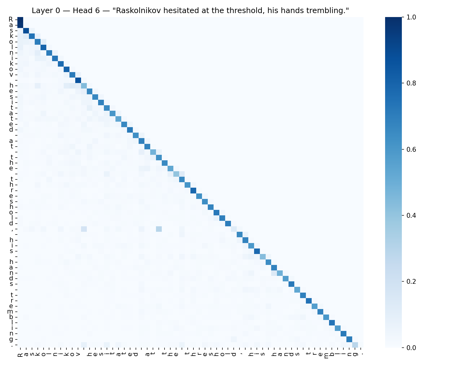
A near-perfect sub-diagonal stripe running the full sequence length without degradation. Every token attends almost exclusively to the token immediately before it. The model's first and most precisely learned behaviour. Six of eight heads in layer 0 are this type. Documented in Elhage et al. 2021 as a foundational component of the induction circuit.
Identity Preservation Head L0_H0
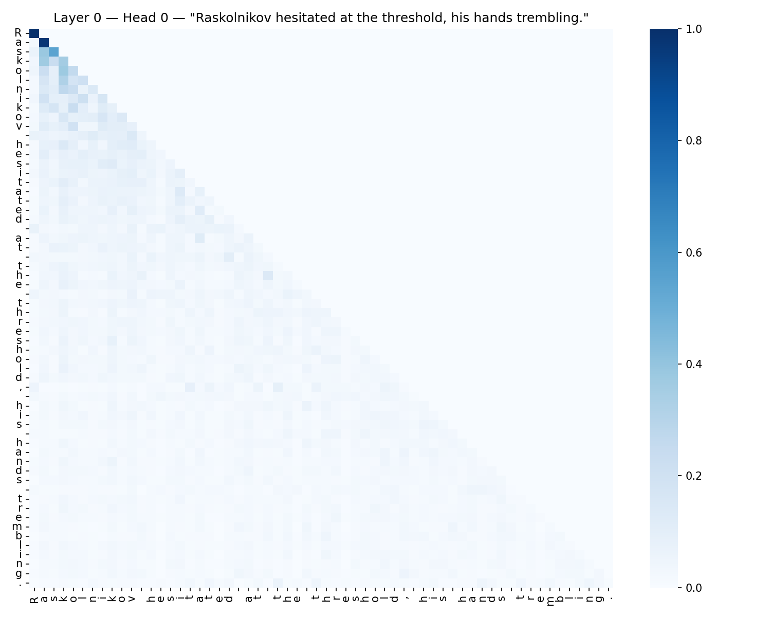
Brightest attention on the main diagonal, with a soft backward wedge fading into recent history. The diagonal degrades progressively for later tokens as competing contextual signals accumulate. Appears exclusively in layer 0 with one secondary appearance in layer 1. Once contextual representations are built, the model has no further use for heads that attend primarily to the token itself.
Word Boundary Head L1_H5
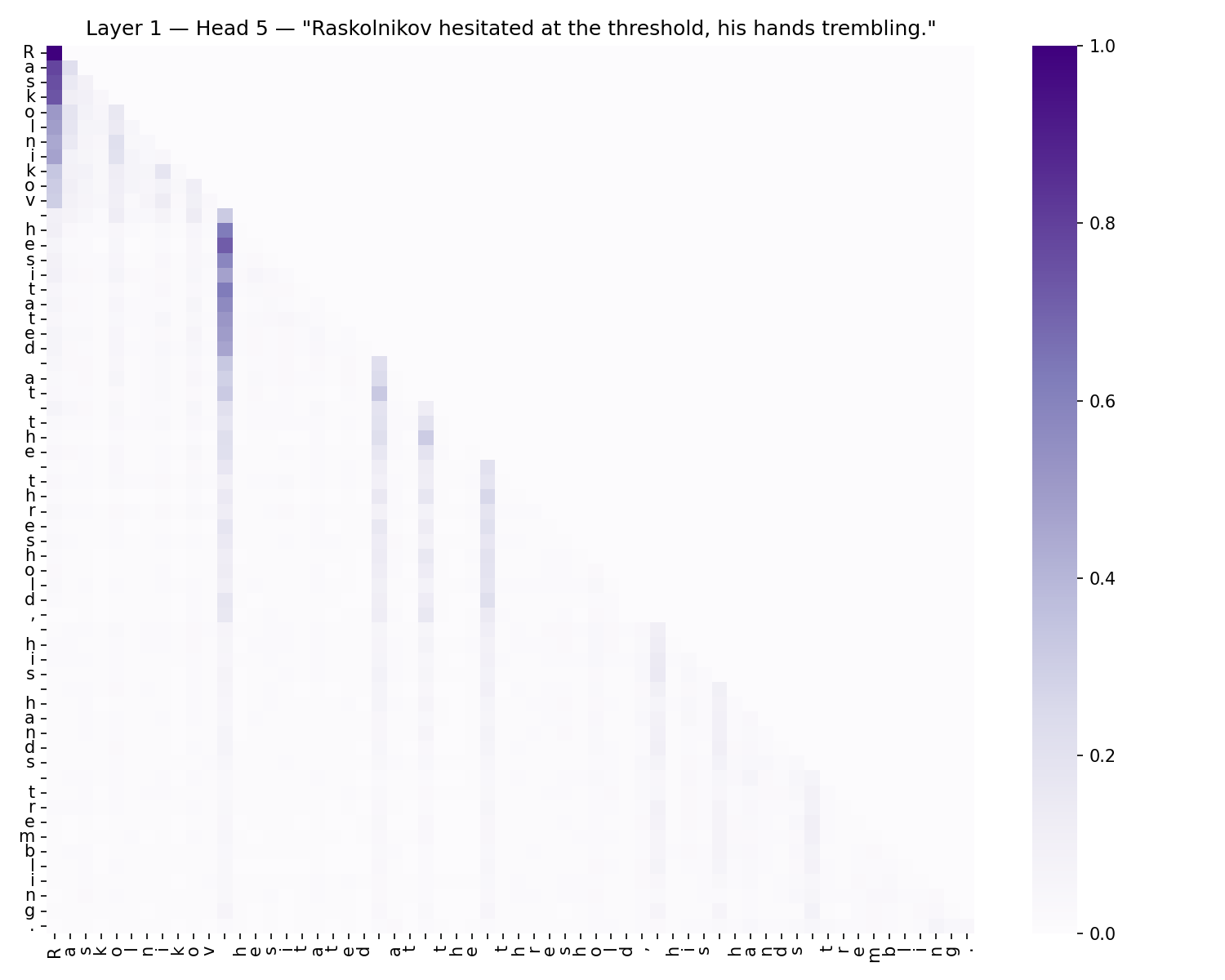
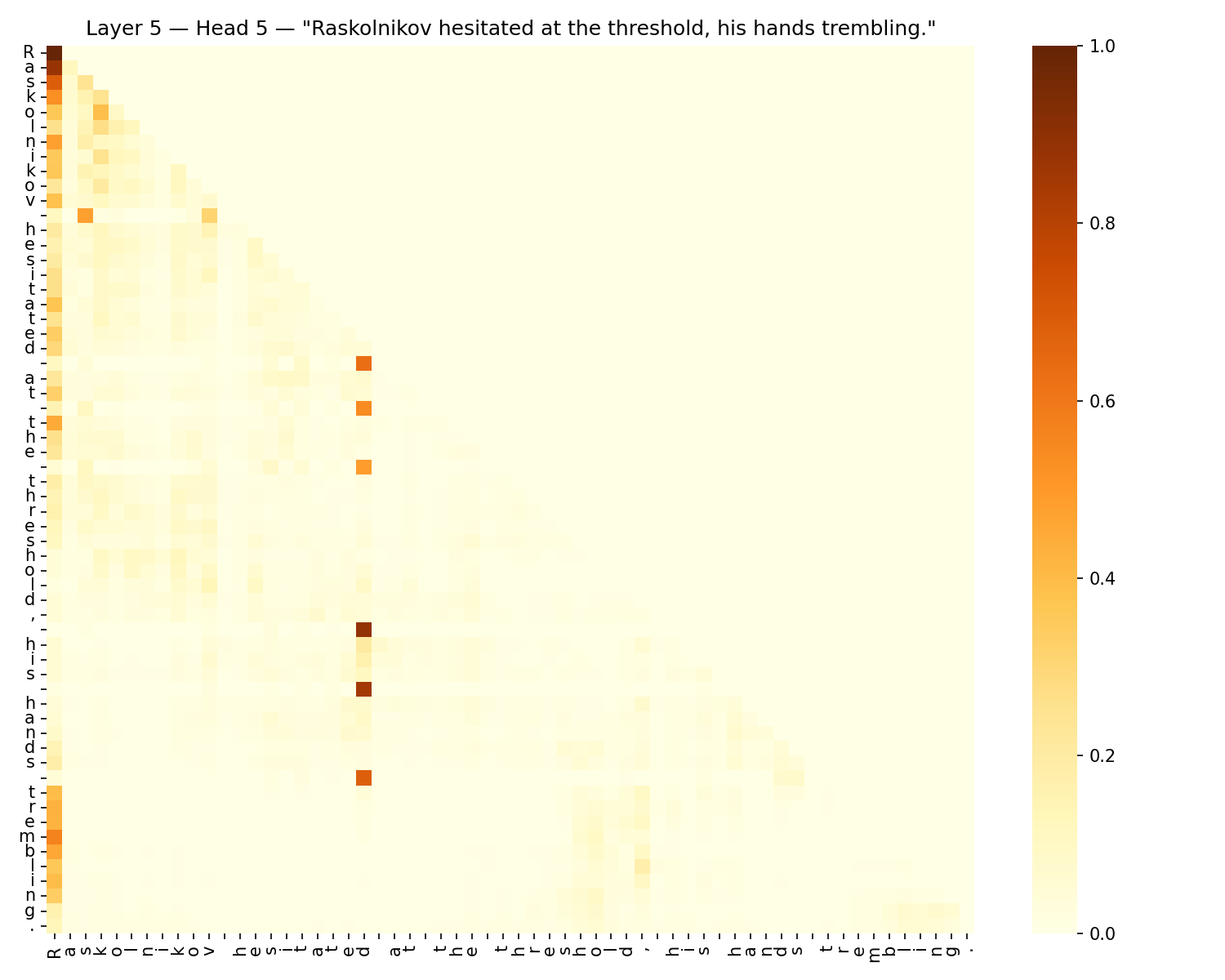
Left: L1_H5, broad boundary head attending to every space. Right: L5_H5, selective boundary head attending to syntactically meaningful spaces only.
Vertical stripes of concentrated attention at space characters. A character-level model with no explicit notion of words independently discovering word-level structure from statistical patterns alone. Two notable findings: word boundary detection is present in every layer from 1 through 7 without exception, and it never centralises into a single unambiguous specialist across all 64 heads. It is a permanently distributed computation. The same circuit type also becomes progressively more selective with depth — early layers attend to the first space only, later layers shift to syntactically meaningful boundary positions.
First Token Sink Head L5_H6, L6_H3
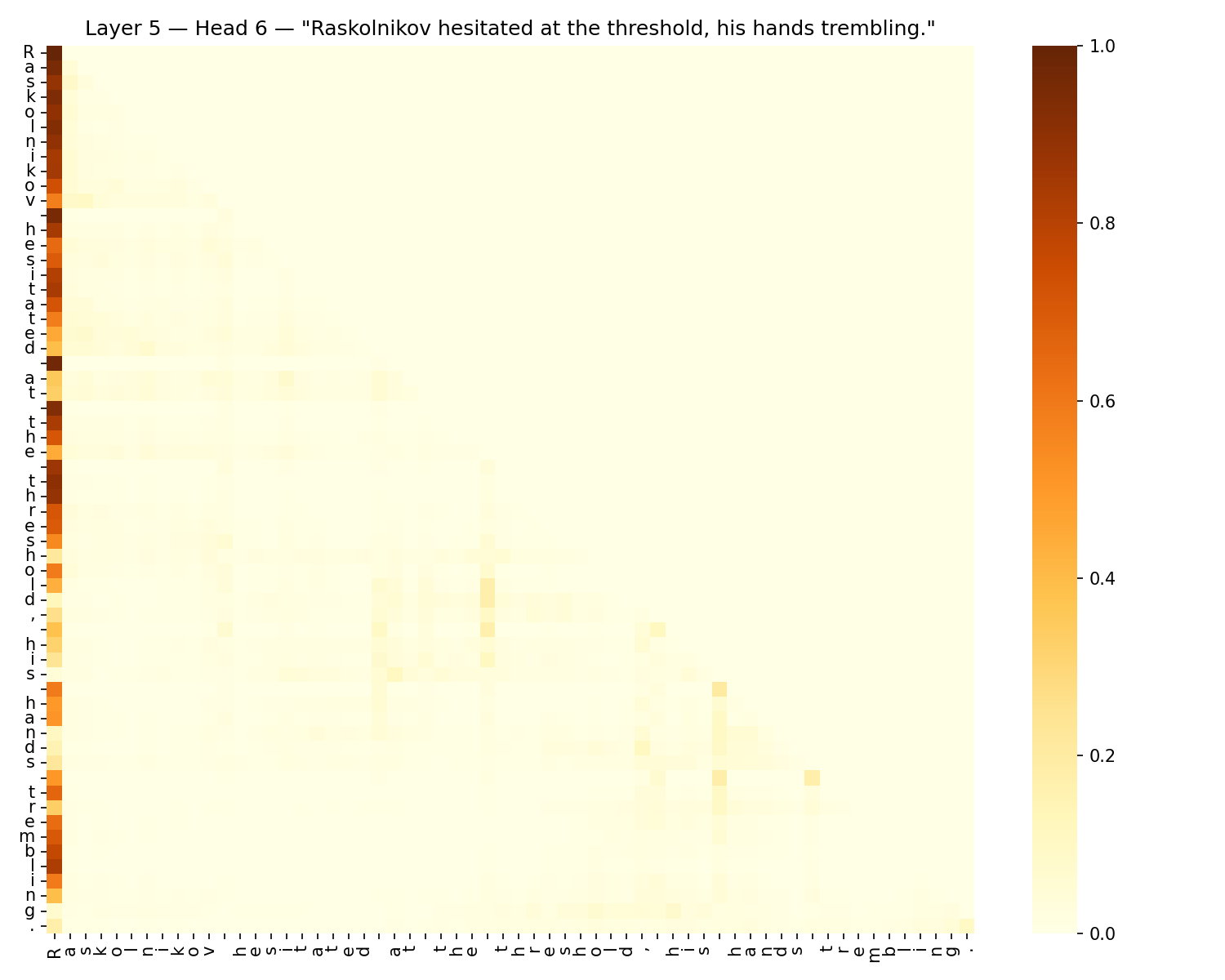
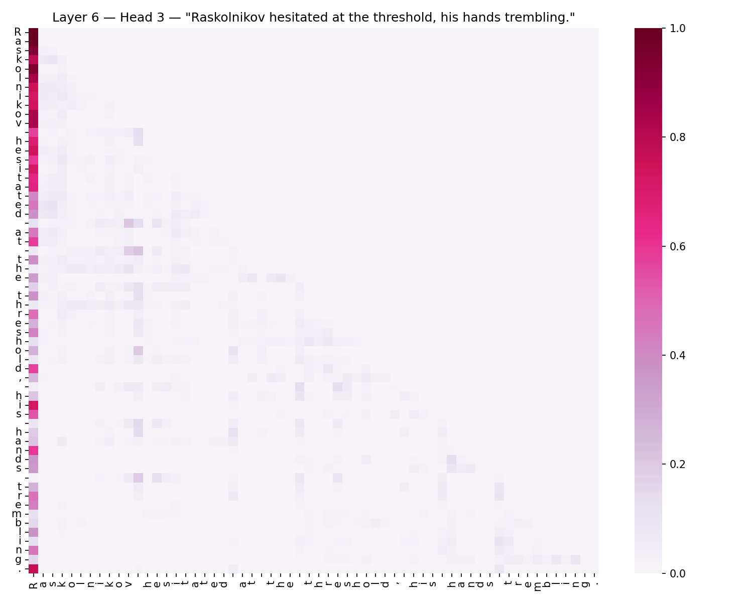
Left: L5_H6, first dedicated sink head at layer 5. Right: L6_H3, strongest sink head in the model at layer 6.
The entire left column is lit. Nearly every token routes strong attention back to the first character regardless of position. This circuit follows a complete lifecycle across the model: weak background signal from layer 1, growing through layers 2 to 4 as a distributed secondary signal in an increasing number of heads, crystallising into dedicated specialist heads at layers 5 and 6, then dispersing back to secondary status at layer 7. Global context aggregation is most active in the middle of the network, not at the end.
Abstract Routing Head L4_H4
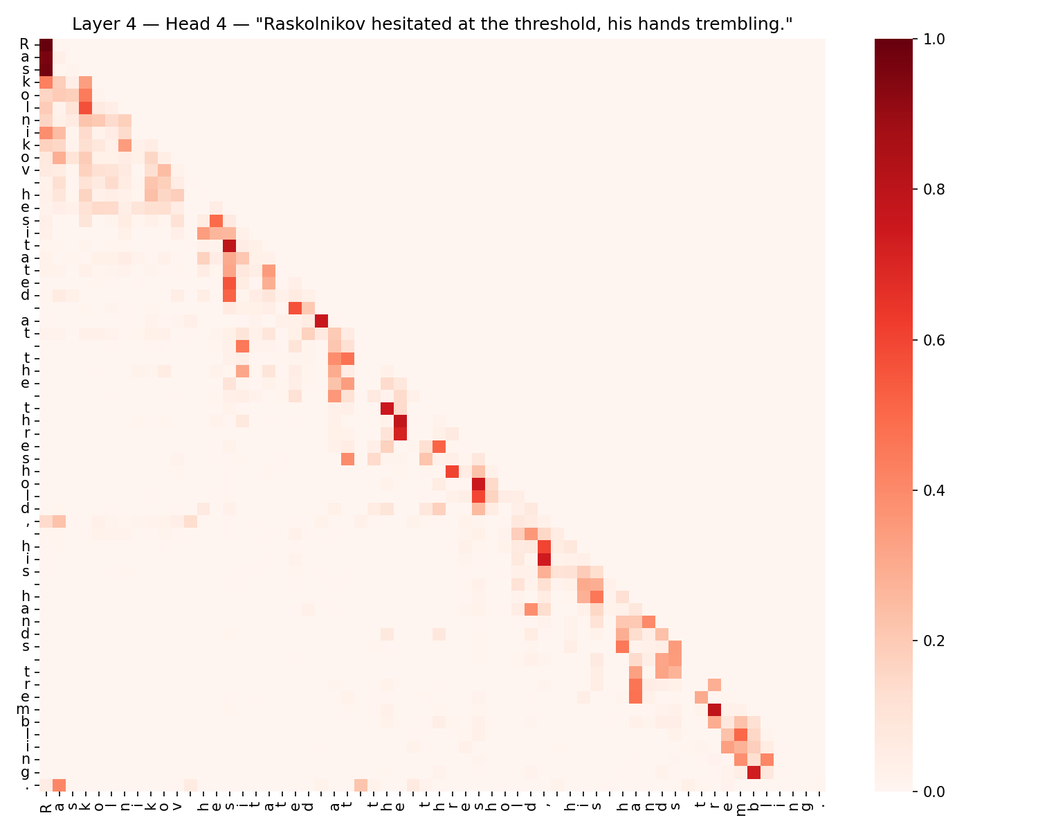
No diagonal. No vertical stripes. Sparse, high-contrast hits at specific non-local positions with the majority of cells near zero. Information is being routed based on learned abstract features, connecting tokens that share semantic or syntactic relevance regardless of distance. L4_H4 is the earliest layer where a strong unambiguous sparse head appears — abstract routing begins earlier than the layer summary alone implies.
Extended Lookback Head L2_H1
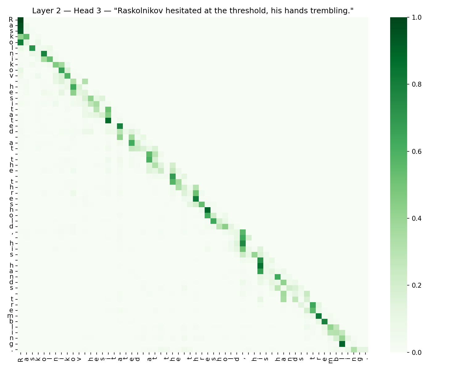
Left: L0_H6, standard previous token head, one step back. Right: L2_H3, extended lookback head, two to three steps back. The stripe moves further from the main diagonal.
Brightest attention sits two to three positions back rather than one, extending the local context window beyond single-step lookback. Its position at layer 2, the final layer before the layer 3 convergence, is the key observation. The model widens its local receptive field immediately before committing to abstract routing.
| Layer | Dominant Type | Character |
|---|---|---|
| 0 | Previous token, identity preservation | Pure local |
| 1 | Previous token, boundary detection emerging | Local with first word boundary signal |
| 2 | Previous token, extended lookback | Local widening before the transition |
| 3 | Abstract routing across all 8 heads | Convergence point, the commit layer |
| 4 | Abstract routing, BOS sink emerging | Abstract dominant, aggregation building |
| 5 | Abstract routing, BOS sink fully formed | Three circuit families running in parallel |
| 6 | Abstract routing, BOS sink peak | Strongest first token sink heads in the model |
| 7 | Abstract routing across all 8 heads | Most functionally committed layer in the model |
Hidden State Analysis — How Token Representations Evolve
The hidden state analysis tracked 8 tokens across all layers using three measurements: norm trajectories (how much information accumulates per token per layer), per-layer norm deltas (where the work is actually being done), and layer-to-layer cosine similarity (whether layers are scaling representations or reorienting them).
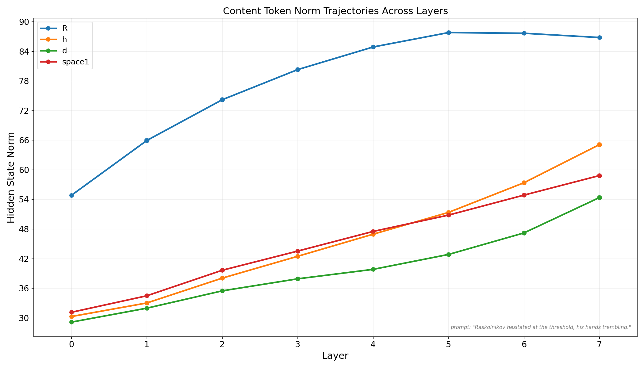
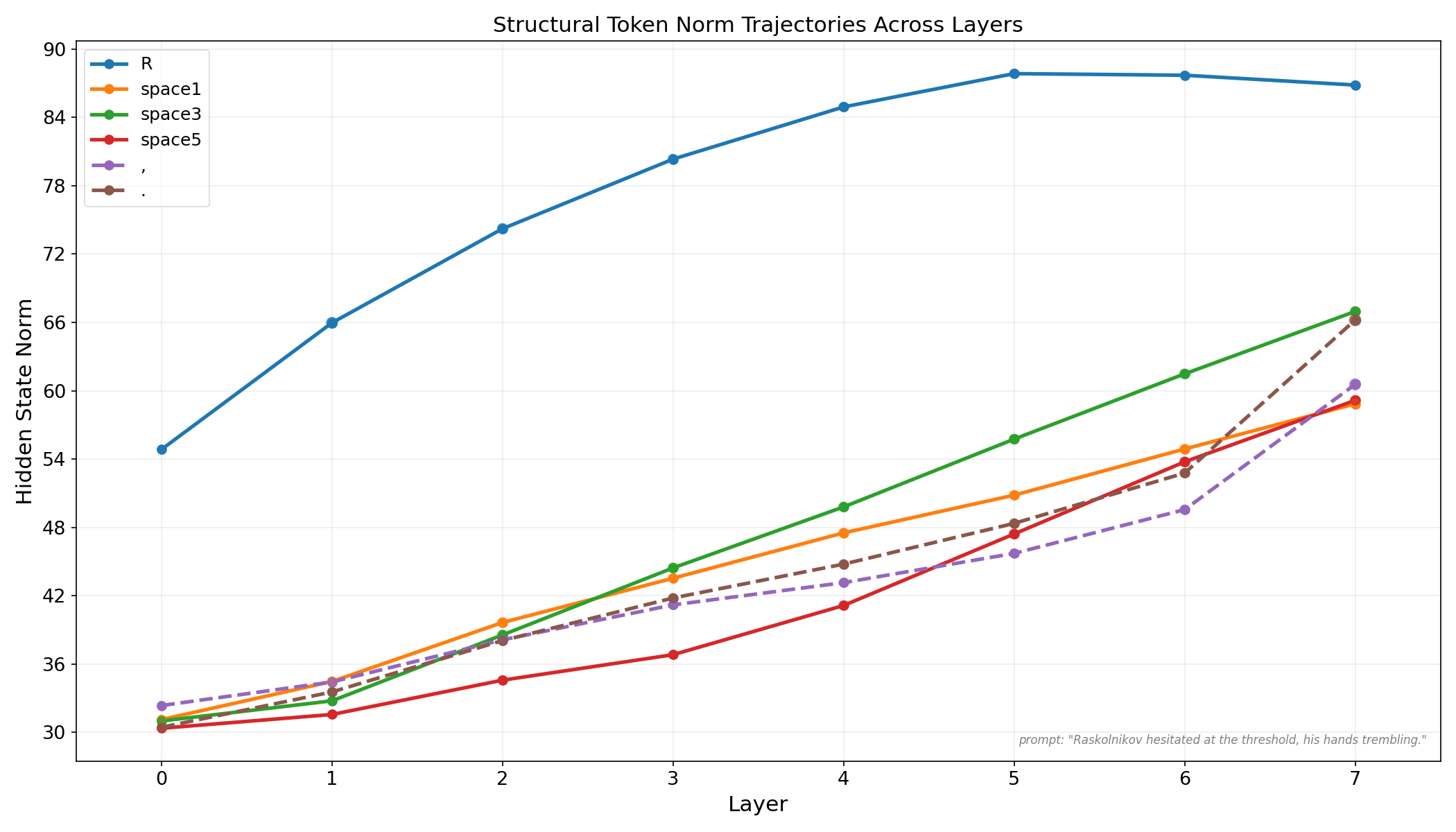
Left: Content token trajectories. R dominates from layer 0 and never yields that lead. Right: Structural token trajectories. The three space tokens diverge despite identical initial embeddings. Punctuation spikes sharply in the final layers.
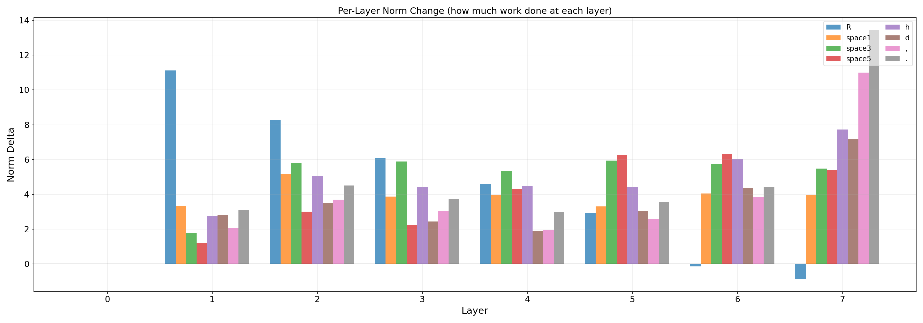
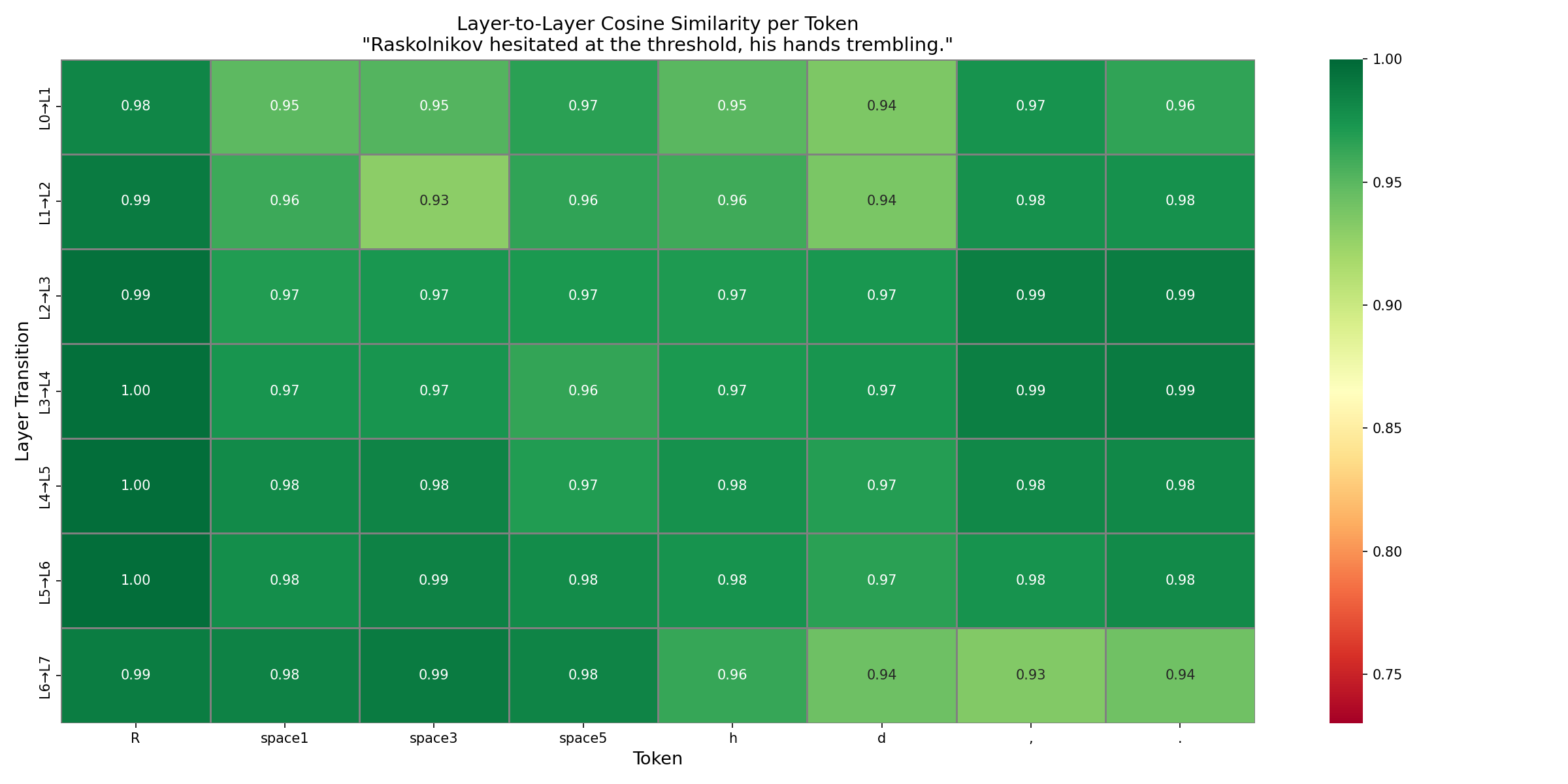
Left: Per-layer norm deltas. R is the only token with negative deltas, at layers 6 and 7. Punctuation's final-layer delta exceeds every other token at every other layer. Right: Cosine similarity heatmap. All values above 0.93 — the model changes direction far less than it changes magnitude. R shows 1.00 across three consecutive middle-layer transitions.
Key findings from the hidden state analysis:
R dominates from layer 0 and redistributes at layer 6. R starts with the highest norm of all tracked tokens and peaks at layer 5. At layer 6 its norm drops for the first time — the only token in the entire analysis to show negative deltas. This is redistribution, not degradation. The model has finished accumulating context into position 0 and begins spreading that information outward toward prediction.
Representational direction stabilises before magnitude. Every cosine similarity value falls between 0.93 and 1.00. The model locks in what tokens mean early and spends subsequent layers building how strongly it represents that meaning. R's direction is fully locked by layer 3, showing 1.00 cosine similarity across three consecutive transitions.
Not all spaces are equal. space3 (before "the"), space1 (after "Raskolnikov"), and space5 (before "his") start with identical embeddings and diverge by the final layer. space3 ends highest. Syntactic role drives representational weight, not token identity.
Punctuation has two distinct phases. Comma and period show anomalously high norm at layer 0, track flat through the middle layers, then spike sharply in the final layers. The final-layer norm delta for punctuation is the largest delta of any token at any layer in the entire analysis. Early layers encode punctuation identity. Final layers encode punctuation function.
The final layer does more directional work than any middle layer. The layer 6 to layer 7 transition shows the lowest cosine similarity values of any transition in the model. The final layer is not polishing settled representations. It is reorienting them.
The attention and hidden state analyses were run independently on the same model and same prompt. Their corroborations are the strongest findings in this project.
The BOS sink circuit timing matches R's norm lifecycle exactly. The first token sink circuit crystallises at layers 5 and 6 in the attention analysis. R's norm peaks at layer 5 and begins declining at layer 6 in the hidden state analysis. Two measurements, same timing, same phenomenon described from different angles.
R's directional lock-in explains why the BOS sink circuit works. R shows 1.00 cosine similarity across three consecutive transitions beginning at layer 3 — its direction is fixed. The BOS sink circuit is stable and reliable precisely because the aggregation target stopped changing direction before the dedicated sink heads fully formed.
The layer 3 convergence appears in both analyses. R's norm delta begins tapering exactly at layer 3, when the attention analysis shows abstract routing committing across all 8 heads simultaneously. The intensive local accumulation phase ends when abstract routing takes command.
Space token divergence matches word boundary head selectivity. Word boundary heads shift from attending to all spaces to attending to syntactically meaningful ones from layer 4 onward. space3, the space that receives the most selective late-layer attention, ends with the highest norm of the three space tokens.
Punctuation processing is a two-stage pipeline. Separator heads appear at layers 3 and 4 in the attention analysis, using punctuation as clause boundaries. The final-layer norm spike for punctuation in the hidden state analysis shows the second stage: building full functional representations when the complete sequence has been processed. Two different computations, two different depths, one consistent story.
The final layer is the sharpest stage in the entire forward pass. Layer 7 is the most functionally committed attention layer in the model. It is also the layer where the largest directional reorientation of token representations occurs and where punctuation receives its largest norm delta. The attention data and the hidden state data agree: the final layer is not cleanup. It is the most specialised processing stage.
For a complete layer-by-layer narrative of what happens during a single forward pass — from raw token embeddings through all 8 layers to the vocabulary projection — read the unified account in research_findings/conclusions.md.
It walks through every layer from input to prediction, weaving the attention and hidden state findings into one coherent story. It is the most complete picture of what NanoLens is actually doing that this project can currently provide.
Single prompt findings. All research findings are from one prompt on one checkpoint. Head classifications and hidden state patterns have not been verified across multiple prompts or training seeds. They are directional observations, not established facts.
Undertrained relative to data recommendations. At 25M parameters and 4.4M characters of training data, NanoLens is approximately 100x below Chinchilla recommendations. The model converges and produces meaningful circuit behaviour, but more data would improve both generation quality and the clarity of learned circuits.
No activation patching. Circuit verification via activation patching is not currently implemented. The findings describe correlational patterns between attention behaviour and hidden state trajectories, not causal mechanisms. Patching is listed under future work in conclusions.md.
Character-level ceiling. Beyond approximately 150M parameters, character-level tokenisation becomes the quality bottleneck. Scaling further requires switching to subword tokenisation.
And as forgotten, Dmitri Fyodorovitch, who has proved, a conscious with the last fraud coffin efforts. He was not to be alarmed, his seemed to go without to, for the the struggle which he recovered himself or it sits the toff and at once am playing to be for shome to be a student place of it? We will trether if you came to
25 million parameters. Character-level. Trained from scratch. Gloriously janky in the best possible way.
Pretrained weights at Releases.
git clone https://github.com/AdityaSinghDevs/nanolens
cd nanolens
pip install -r requirements.txt
Verify setup:
python cli.py -dTrain from scratch:
python cli.pyGenerate:
python cli.py --checkpoint checkpoints/nanolens_v1.pt -gInspect attention patterns:
python cli.py --checkpoint checkpoints/nanolens_v1.pt \
              -i "Raskolnikov hesitated at the threshold." -aw
Inspect hidden states:
python cli.py --checkpoint checkpoints/nanolens_v1.pt \
              -i "Raskolnikov hesitated at the threshold." -hs
Both in one pass:
python cli.py --checkpoint checkpoints/nanolens_v1.pt \
              -i "Raskolnikov hesitated at the threshold." -aw -hs
For full training configuration, hyperparameter guide, scaling mathematics, hardware ceiling estimates, and CLI reference: TRAINING.md
Pretrained checkpoint: Releases
mv nanolens_v1.pt checkpoints/nanolens_v1.pt
python cli.py --checkpoint checkpoints/nanolens_v1.pt -g
8 layers, 8 heads, 512 embedding dim, 5000 steps, 4.4M characters of Dostoevsky. Final val loss 1.1144. Size: ~113MB.
nanolens/
├── config/
│   └── default.yaml             # all hyperparameters, nothing hardcoded
├── nanolens/
│   ├── data/
│   │   ├── training/            # drop your .txt files here
│   │   ├── tokenizer.py         # character-level encode/decode
│   │   └── loader.py            # batching, train/val split
│   ├── model/
│   │   ├── head.py              # single attention head
│   │   ├── attention.py         # multi-head attention
│   │   ├── ffwd.py              # feedforward block
│   │   ├── blocks.py            # full transformer block
│   │   └── transformer.py       # full model + generate()
│   ├── training/
│   │   ├── optimizer.py         # AdamW with param group separation
│   │   └── trainer.py           # training loop + LR decay + checkpointing
│   ├── inference/
│   │   └── generate.py          # generation wrapper
│   └── analysis/
│       ├── inspector.py         # dual-mechanism inspection
│       └── visualize.py         # all plots
├── results/
│   ├── attention/               # heatmaps, L{layer}_H{head}.png
│   └── hidden_states/           # norm trajectories, cosine similarity
├── research_findings/
│   ├── attention_circuit_analysis.md
│   ├── hidden_state_analysis.md
│   └── conclusions.md
├── TRAINING.md                  # configuration, scaling, CLI reference
├── cli.py                       # entry point
├── requirements.txt
└── README.md
If NanoLens is useful for your research, teaching, or learning, a star on the repo helps it reach more people. If you train your own model and find interesting circuit behaviour, open an issue or reach out — genuinely curious what other architectures and datasets produce.
- Vaswani et al. — Attention Is All You Need
- Elhage et al. — A Mathematical Framework for Transformer Circuits
- Andrej Karpathy — Let's build GPT: from scratch, in code, spelled out
- Neel Nanda — TransformerLens
MIT — see LICENSE for details.